머신러닝과 딥러닝(12)_파이토치로 구현한 논리회귀

카테고리 없음

by teminam 2023. 6. 16. 09:07

1. 단항 논리 회귀 실습

논리 회귀(Logistic Regrssion)
분류를 할 때 사용하며 선형 회귀 공식으로부터 나왔기 때문에 논리 회귀라는 이름이 붙여짐

> 직선 하나(선형 회귀)를 사용해서 예측한다면 제대로 예측할 수 없음

> Sigmoid 함수(Logistic 함수)를 사용하여 정확도를 높임

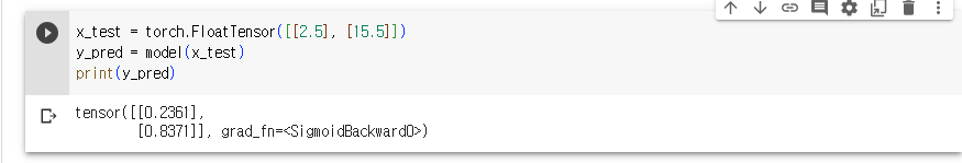
Sigmoid 함수

예측값을 0에서 1사이 값이 되도록 만듬
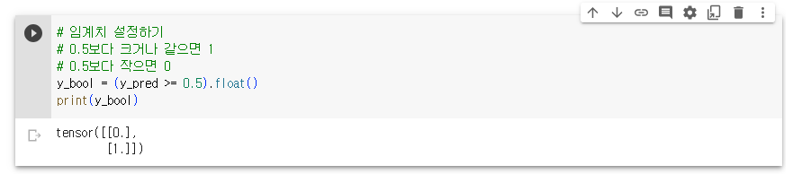
0에서 1사이의 연속된 값을 출력으로 하기 때문에 보통 0.5를 기준으로 구분

비용 함수

논리 회귀에서는 nn.BCELoss() 함수를 사용하여 Loss를 계산
Binary Cross Entropy

epochs = 1000

for epoch in range(epochs + 1):
  y_pred = model(x_train)
  loss = nn.BCELoss()(y_pred, y_train)
  optimizer.zero_grad()
  loss.backward()
  optimizer.step()

  if epoch % 100 == 0:
    print(f'Epoch {epoch}/{epoch} Loss: {loss:.6f}')

2. 다항 논리회귀 실습

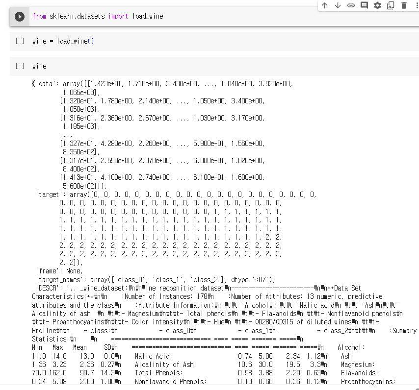
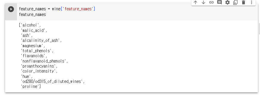
3. 와인 품종 예측해보기

sklearn.datasets.load_wine 데이터셋은 이탈리아의 같은 지역에서 재배된 세가지 다른 품종으로 만든 와인을 화학적으로 분석한 결과

문제

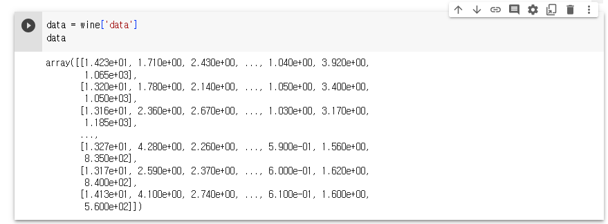
13개의 성분을 분석하여 어떤 와인인지 맞춰보자
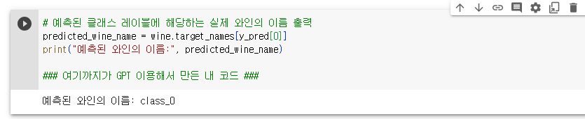
단, 트레이닝 데이터를 80%, 테스트 데이터를 20%로 하며 테스트 데이터의 0번 인덱스가 어떤 와인인지 출력하고, 테스트 정확도도 출력

# https://scikit-learn.org/stable/modules/generated/sklearn.datasets.load_wine.html#sklearn.datasets.load_wine 에서 갖고온 그냥 예시 코드임
# Author: Virgile Fritsch <virgile.fritsch@inria.fr>
# License: BSD 3 clause

import numpy as np
from sklearn.covariance import EllipticEnvelope
from sklearn.svm import OneClassSVM
import matplotlib.pyplot as plt
import matplotlib.font_manager
from sklearn.datasets import load_wine

# Define "classifiers" to be used
classifiers = {
    "Empirical Covariance": EllipticEnvelope(support_fraction=1.0, contamination=0.25),
    "Robust Covariance (Minimum Covariance Determinant)": EllipticEnvelope(
        contamination=0.25
    ),
    "OCSVM": OneClassSVM(nu=0.25, gamma=0.35),
}
colors = ["m", "g", "b"]
legend1 = {}
legend2 = {}

# Get data
X1 = load_wine()["data"][:, [1, 2]]  # two clusters

# Learn a frontier for outlier detection with several classifiers
xx1, yy1 = np.meshgrid(np.linspace(0, 6, 500), np.linspace(1, 4.5, 500))
for i, (clf_name, clf) in enumerate(classifiers.items()):
    plt.figure(1)
    clf.fit(X1)
    Z1 = clf.decision_function(np.c_[xx1.ravel(), yy1.ravel()])
    Z1 = Z1.reshape(xx1.shape)
    legend1[clf_name] = plt.contour(
        xx1, yy1, Z1, levels=[0], linewidths=2, colors=colors[i]
    )

legend1_values_list = list(legend1.values())
legend1_keys_list = list(legend1.keys())

# Plot the results (= shape of the data points cloud)
plt.figure(1)  # two clusters
plt.title("Outlier detection on a real data set (wine recognition)")
plt.scatter(X1[:, 0], X1[:, 1], color="black")
bbox_args = dict(boxstyle="round", fc="0.8")
arrow_args = dict(arrowstyle="->")
plt.annotate(
    "outlying points",
    xy=(4, 2),
    xycoords="data",
    textcoords="data",
    xytext=(3, 1.25),
    bbox=bbox_args,
    arrowprops=arrow_args,
)
plt.xlim((xx1.min(), xx1.max()))
plt.ylim((yy1.min(), yy1.max()))
plt.legend(
    (
        legend1_values_list[0].collections[0],
        legend1_values_list[1].collections[0],
        legend1_values_list[2].collections[0],
    ),
    (legend1_keys_list[0], legend1_keys_list[1], legend1_keys_list[2]),
    loc="upper center",
    prop=matplotlib.font_manager.FontProperties(size=11),
)
plt.ylabel("ash")
plt.xlabel("malic_acid")

plt.show()

print(wine['DESCR'])

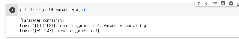
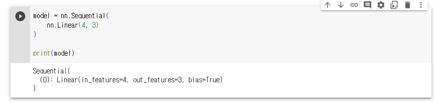
model = nn.Sequential(
    nn.Linear(13, 3)
)

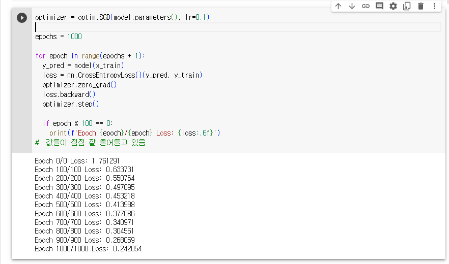
optimizer = optim.Adam(model.parameters(), lr=0.01)

epochs = 1000

for epoch in range(epochs + 1):
    y_pred = model(x_train)
    loss = nn.CrossEntropyLoss()(y_pred, y_train)

    optimizer.zero_grad()
    loss.backward()
    optimizer.step()

    if epoch % 100 == 0:
        y_prob = nn.Softmax(1)(y_pred)
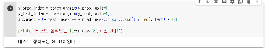
        y_pred_index = torch.argmax(y_prob, axis=1)
        y_train_index = torch.argmax(y_train, axis=1)
        accuracy = (y_train_index == y_pred_index).float().sum() / len(y_train) * 100
        print(f'Epoch { epoch:4d}/{epochs} Loss: {loss:.6f} Accuracy: {accuracy:.2f}%')

        # 정확도가 낮은걸 보니, 경사하강법을 사용하자.
        # SGD 에서 Adam으로 바꾸니 정확도가 확 올라감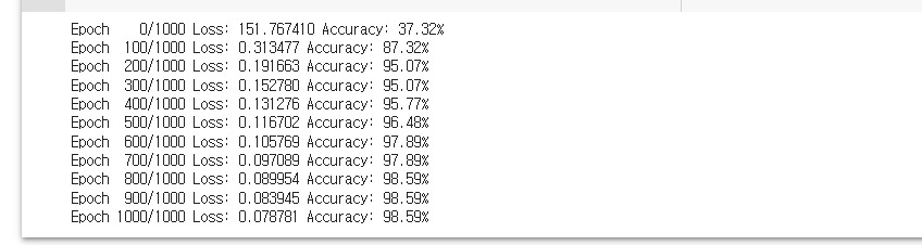

4. 경사하강법의 종류

4-1. 배치 경사하강법

가장 기본적인 경사하강법(Vanilla Gradient Descent)
데이터셋 전체를 고려하여 손실함수를 계산
한 번의 Epoch에 모든 파라미터 업데이트를 단 한번만 수행
Batch의 개수와 Iteration은 1이고, Batch size는 전체 데이터의 개수
파라미터 업데이트할 때 한 번에 전체 데이터셋을 고려하기 때문에 모델 학습시 많은 시간과 메모리가 필요하다는 단점

4-2. 확률적 경사하강법

확률적 경사하강법은 배치 경사하강법(Stochastic Gradient Descent)이 모델 학습시 많은 시간과 메모리가 필요하다는 단점을 계산하기 위해 제안된 기법
Batch size를 1로 설정하여 파라미터를 업데이트 하기 때문에 배치 경사하강법 보다 훨씬 빠르고 적은 메모리로 학습이 진행
파라미터 값의 업데이트 폭이 불안정하기 때문에 정확도가 낮은 경우가 생길 수 있음
SGD가 여기에 포함됨